VIMOS UBVRI zero-points

Executive summary: After a quick reduction of the VIMOS imaging data from the first commissioning run, the photometric zero-points are found to be approximately:

	A3	B1
U	25.77	25.85
B	27.61	27.62
V	27.35	27.45
R	27.47	27.53
I	26.63	26.68

The gains of the two CCDs used on this run were found to be:

A3 1.65 e-/ADU

B1 1.50 e-/ADU

The data from the first commissioning data was overscan corrected, bias subtracted and flat fielded in the usual way. Only the imaging data (2Kx2K sub-raster) was reduced. The image section [1:50,*] was used as the overscan region. There were only a small number of bias frames available for the imaging data. Almost all the flats taken were used, despite the large number of star trails and out-of-focus stars in several of them. They were combined using a median which should get rid these defects. A better set of flats will be generated in the future incorporating some of the deeper imaging data (with the sources removed) as well.

To determine the gain, statistics were computed on a number 100x100 pixel subrasters of all the images. For each subraster, the average (in ADU's) was compared to the standard deviation. The relation between signal (S) and noise (N) in electrons in a blank (sky dominated) section of sky should be:

Where R is the read noise (in electrons) and g is the gain (in units of e-/ADU). Gain is the conversion factor between e- and ADU the equation in ADU looks like:

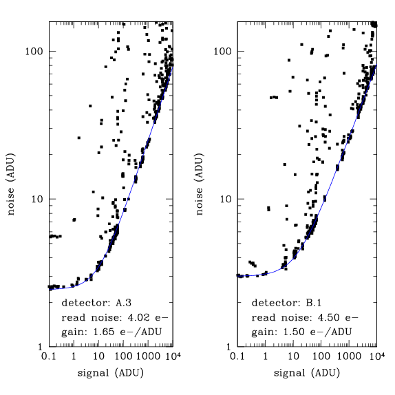
Note that the gain does not factor out of this relation. This means that if one plots N(ADU) vs S(ADU), it is possible to determine the gain and the read noise. At low signal, read noise dominates, and can be simply read off the graph. At high signal, the read noise can be neglected the gain be determined by fitting. The slope of the relation is still one 0.5 on a log-log plot, but with offset due the gain. The above equation becomes:

or taking the log:

The figure at right shows the noise in ADU plotted against signal in ADU for a large number of sub-rasters. The blue curves show the fit. The points lying above the curve are derived from sub-rasters which are not all sky (ie, the have some objects in them) and therefore have a higher standard deviation.

The zero-points were determined using measurements of flux from the Landolt standard stars. I have assumed that all such observations were taken under photometric conditions. Because of the small range in airmass of the observations, I have used the measurements of the airmass coefficients given at http://www.eso.org/paranal/sv/html/data/photom.html They are summarized here:

Filter	extinction coefficient
U	0.495
B	0.258
V	0.172
R	0.131
I	0.073

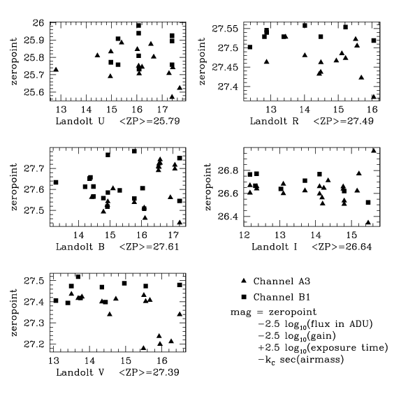
The figure at right shows the zero points determined for each star plotted as a function of Landolt magnitude. The means for each filter are also shown. Here, the two channels have been averaged together, which may not always be appropriate. The equation describing the zero-point explicitly includes the gain.

Caveats

There were only 3 bias frames for each channel available in imaging mode. This may increase the apparent read noise.
Similarly, the flats may have to much noise in them. This is more serious, as it will affect the measurement of the gain and hence zero-points. Further, the gain may have changed during the observations due to modifications to the read out setup. This was not taken into consideration in the above calculation.
Since no observing log was available to me, I have included all observation that seemed be of Landolt standards. The only exception is frames that completely lacked a WCS.
The zero-points given are for ``outside the atmosphere'', that is corrected to 0 airmass. It may be necessary to account for airmass in order to compare these results with other derivations of the zero-points
Colour terms were not included in the determination of the zero-points

Send comments/suggestions/problems to
Stephen.Gwyn@astrsp-mrs.fr